Topic Classification of Texts Locally Using BERTopic

I’ve been recently working on survey response data that in addition to aggregatable question types like Likert-scale and multiple-choice questions, includes optional free-text questions. Although we are lucky that thousands of the respondents spend time elaborating on questions and leaving comprehensive free-text responses, getting insights from these text responses is challenging.

While investigating how to enrich this text data with proper metadata related to their topics, I came across BERTopic which introduces itself as a topic modeling technique to create clusters allowing for easily interpretable topics. In this post, I’ll explore BERTopic and will go through an example to explain what adjustments worked for me.

BERTopic

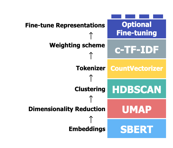
BERTopic leverages a few popular NLP and clustering algorithms and libraries to classify raw texts into meaningful topics. It reshapes the texts in a sequence of steps, including embedding, dimensionality reduction, clustering, tokenization, and weighting words (explained in more detail in its docs ):

BERTopic is fundamentally built upon BERT embeddings, one of the leading NLP techniques. While traditional topic modeling techniques, like LDA rely on probabilistic graphical models to identify topics, BERTopic uses the rich, contextual embeddings from BERT to cluster similar texts. This offers two main advantages:

1. Contextual Understanding: BERT’s deep understanding of context means that words with multiple meanings can be more appropriately clustered based on their actual usage in texts, leading to more accurate topic allocations.
2. Flexibility: BERTopic is not just confined to English. Thanks to the multilingual capabilities of BERT, it can be adapted for several languages without significant changes in the approach.

The choice of BERTopic over traditional methods largely depends on the specific requirements of a project, but its modern and deep learning-based approach can often yield more nuanced and contextually relevant results.

Installing the library and preparing the sample data

Start by installing the required Python libraries and importing them:

pip install bertopic sentence-transformers pandas scikit-learn

import pandas as pd
from bertopic import BERTopic
from sentence_transformers import SentenceTransformer
from sklearn.feature_extraction.text import CountVectorizer
import pickle

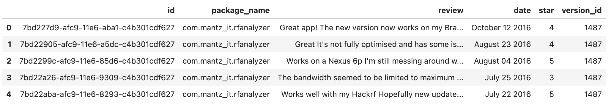
I will use the app reviews dataset from Android Apps and User Feedback project published by researchers at the University of Zurich. This dataset consists of 288K reviews extracted from Google Play, but as it makes more sense to limit this exercise to one single app and see the topics of reviews submitted for it, I have picked Telegram:

df_orig = pd.read_csv("reviews.csv")
df_orig.head()

## filtering data on Telegram
df = df_orig[df_orig["package_name"] == "org.telegram.messenger"]

## Getting rid of reviews like 'nice', 'good', etc by keeping only the reviews with at least 10 words
df["n_words"] = df["review"].apply(lambda x: len(x.split(" ")))
df = df[df["n_words"] >= 10]

Generating and storing Embeddings

The first step in clustering our text data is to convert them to some sort of numerical representation. This can be done using publicly available models, and BERTopic uses the famous sentence-transformers library in this step of the process. If you’re interested in knowing more about how sentence-transformers works, check out their docs or take a look at my blog post which is a brief explanation of how to use this library for embedding texts locally.

We don’t necessarily need to import sentence-transformers and do the embeddings step outside the topic generation step as it’s managed by the BERTopic library behind the scenes. But since this is a computationally costly process, we will generate the embeddings once and will store them in our machine’s memory or disk, and pass it to our topic generation model as many times as we want. This will enable us to experiment with various hyperparameters of BERTopic quickly and conveniently.

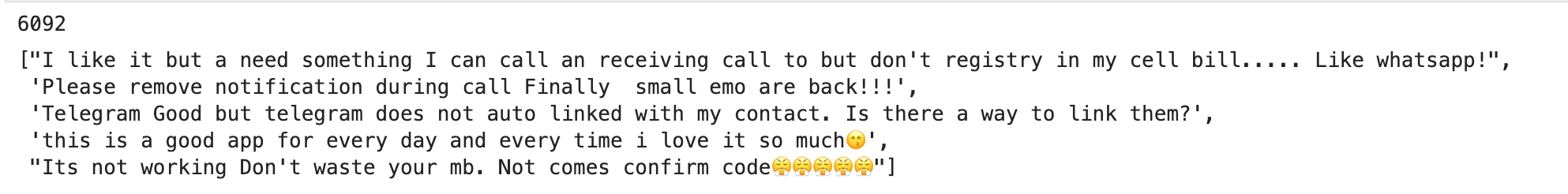
docs = df["review"].values.tolist()
print(len(docs))
docs[:5]

## Pre-calculating embeddings
embedding_model = SentenceTransformer("all-MiniLM-L6-v2")
embeddings = embedding_model.encode(docs, show_progress_bar=True)

## Storing embeddings on the disk
with open("embeddings.pkl", "wb") as f:
    pickle.dump(embeddings, f)

## We can load the stored embeddings later on if needed
with open("embeddings.pkl", "rb") as f:
    embeddings = pickle.load(f)

Classify reviews into topics

We have another optional but beneficial step before generating topics. In my first attempt to classify texts into topics using BERTopic, meaningless words like “in, an, at, for, etc” had a significant presence in topic representations and some of the final categories had no semantic meaning. We can ask BERTopic to skip these words (which are called stopwords in the NLP world) by creating a vectorizer model and passing it to our topic generation model:

vectorizer_model = CountVectorizer(stop_words="english", ngram_range=(1, 1))

Use the following instead if you want to add some custom stopwords to be skipped:

from nltk.corpus import stopwords


default_stopwords = stopwords.words("english")
custom_stopwords = ["my", "custom", "list", "of", "words"]
stopwords_all = default_stopwords + custom_stopwords

vectorizer_model = CountVectorizer(stop_words=stopwords_all, ngram_range=(1, 1))

Here I’m using the default value for ngram_range (so it can also be dropped from the above code). ngram_range is used to determine the range of n-grams extracted by our topic generation model. In simple terms, if we have so many words with two or more words (like New York, tech debt, etc) and we want to capture them accordingly, ngram_range should probably be set to (1, 2) for example, but I experimented with this and final results always seemed more useful with ngram_range=(1, 1).

Now let’s classify the texts into topics:

topic_model = BERTopic(
  # Pipeline models
  embedding_model=embedding_model,
  vectorizer_model=vectorizer_model,

  # Hyperparameters
  top_n_words=10,
  verbose=True
)
topics, probs = topic_model.fit_transform(documents=docs, embeddings=embeddings)

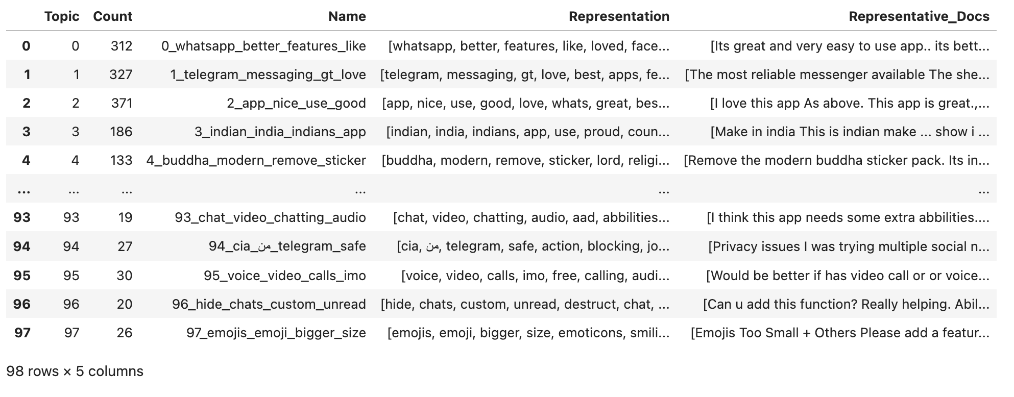
topic_model.get_topic_info()

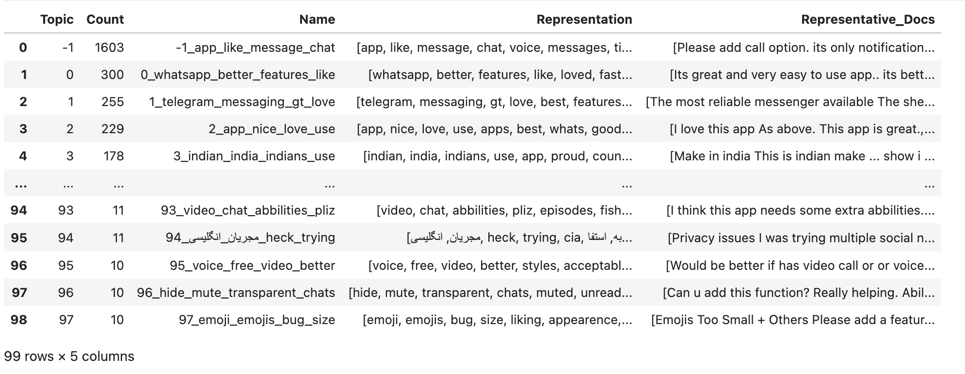
So we have 100 topics, but let’s see what pieces of information we have for each topic:

• Topic: A numerical ID for each topic. As you see in the picture above, the numbers start from -1. The texts in the -1 topic are not related to each other in a meaningful way, and the only reason they are in the same bucket is that BERTopic hasn’t been able to find proper topics for them.
• Count: Number of texts (rows in the dataframe) that are classified into this topic.
• Name: Numerical ID of the topic combined with the four most occurring words in this topic.
• Representation: These are the words that occur most often in the texts classified in this topic. The number of words in this list is determined by the top_n_words parameter above and it has a default value of 10. It is recommended to keep it low, otherwise you’ll get so few items classified in each topic and the number of outliers will increase.
• Representative_Docs: List of the texts that are classified into this topic.

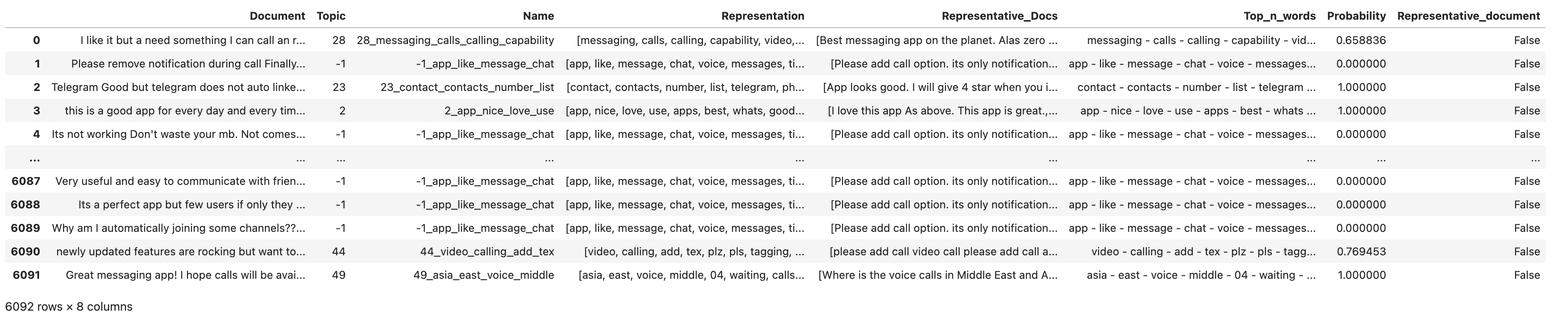
To get a more practical view of how each text has been classified, we can use:

topic_model.get_document_info(docs)

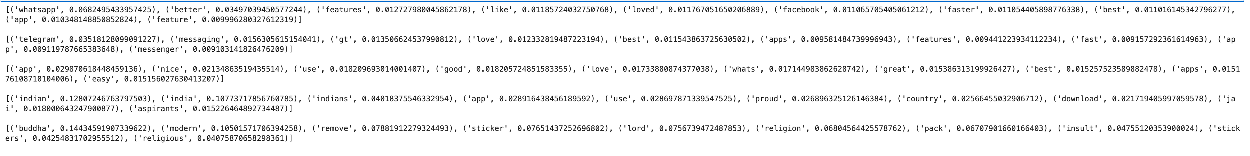
And what are the representations (top words) of our main topics?

for i in range(5):
    print(topic_model.get_topic(i), "\n")

Finally, we can save our topic model to re-use later without computing them from scratch:

topic_model.save("topic-model", serialization="safetensors", save_ctfidf=True, save_embedding_model=embedding_model)

## Later load it with:
BERTopic.load("topic-model")

Reducing outliers

As we saw earlier, a significant number of texts have been classified as outliers (which means they don’t have any topics assigned to them). Upon manually examining a few of these outliers, they seemed to belong to one of the topics if we don’t want to be very strict about our criteria. BERTopic provides a simple way for reducing these outliers and re-assigning them to our existing topics:

new_topics = topic_model.reduce_outliers(documents=docs, topics=topics, strategy="embeddings", embeddings=embeddings)
topic_model.update_topics(docs=docs, topics=new_topics, vectorizer_model=vectorizer_model)

topic_model.get_topic_info()

There is no -1 topic anymore and all of the texts belong to one of the topic classifications now. Here I’ve used the embeddings strategy, but there are other strategies explained in BERTopic’s documentation .

Conclusion

In wrapping up, topic modeling is an incredibly powerful tool for extracting insights from large volumes of text data. With advancements in natural language processing, tools like BERTopic are making this task not only more accurate but also more interpretable. As we’ve walked through in this post, setting up and using BERTopic is relatively straightforward, and its adaptability means it can be fine-tuned for various datasets and requirements. If you’re dealing with a sizeable text dataset and are keen to unearth the hidden topics within, BERTopic is undoubtedly worth a try.

There are a bunch of hyperparameters that can be tweaked to improve the results, but in the end, it mainly depends on the use cases and what we’re trying to achieve. I’ll be experimenting more with BERTopic in the future, so let me know if you have a question you want to be answered about this approach for classifying texts.

Comment? Reply via Email, Mastodon or Twitter.